多目标跟踪中的数据关联代码实践(上)


前言

接下来我们将对多目标跟踪任务中的数据关联算法进行研究,我将结合一些文献和自己的理解,利用一些工具对相关数据关联算法进行实验,包括基于IOU的贪婪匹配、基于匈牙利和KM算法线性偶图匹配、基于图论的离线数据关联(主要介绍最小代价流)以及最新的一些基于深度学习的端到端数据关联网络。代码我都会随博客一起发到github

1 背景简介

之前我们也说到,目前主流的MOT框架是DBT框架,这种框架的特点就是离不开数据关联算法,不论是对不同帧之间跟踪轨迹的关联还是跟踪轨迹和观测量的关联, 有数据关联才能更好的保证目标ID的连续性。数据关联算法以偶图匹配类为主,尤其是在离线跟踪中存在有大量基于图论的算法,比如:最小代价流、最大流、最小割、超图等等。而近两年也出现了一批端到端的数据关联算法,对于这一点呢,有几个很大的问题,一个是数据关联是一个n:m的问题,而网络对于输出的尺寸一般要求是固定的,如果构建关联矩阵是一个问题。另外,数据关联从理论上来讲是一个不可导的过程,其包含有一些排序的过程,如何处理这一点也很重要。

2 基于IOU的贪婪匹配

2.1 IOU Tracker & V-IOU Tracker

不得不说IOU Tracker和他的改进版V-IOU Tracker算是多目标跟踪算法中的一股清流,方法特别简单粗暴,对于检测质量很好的场景效果比较好。首先我们交代一下IOU的度量方式:

$$ IOU\left( {a,b} \right) = \frac{{Area\left( a \right) \cap Area\left( b \right)}}{{Area\left( a \right) \cup Area\left( b \right)}} $$
IOU Tracker的跟踪方式没有跟踪,只有数据关联,关联指标就是IOU,关联算法就是一种基于IOU的贪婪匹配算法:

image-20200305162120637

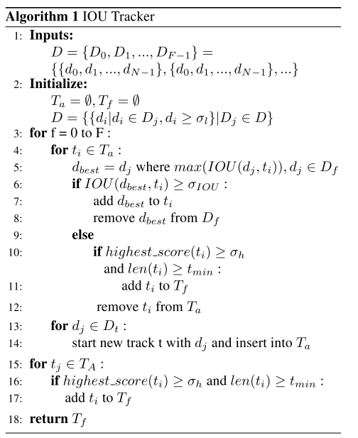
这里我们留到下一节将,我会利用不同的贪婪方式进行IOU匹配。那么V-IOU的改进就是,由于IOU Tracker仅仅是对观测量进行了关联,当目标丢失或者检测不到的时候,便无法重建轨迹,因此V-IOU加入了KCF单目标跟踪器来弥补这一漏洞,也很粗暴。。

2.2 IOU Matching

基于贪婪算法的数据关联的核心思想就是,不考虑整体最优,只考虑个体最优。这里我设计了两种贪婪方式,第一种Local IOU Matching,即依次为每条跟踪轨迹分配观测量,只要IOU满足条件即可,流程如下:

image-20200305162851792

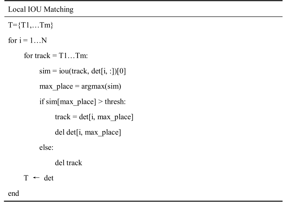
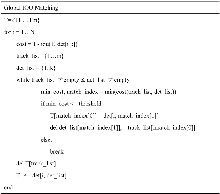
IOU Tracker就是采用的这种局部贪心方式,这种贪心策略的特点是每次为当前跟踪轨迹选择与之IOU最大的观测量。那么我们再提出一种全局的贪婪策略,即每次选择所有关联信息中IOU最大的匹配对,流程如下:

image-20200305170556313

这两种贪婪方式的代码如下:

1
2
3
4
5
6
7
8
9
10
11
12
13
14
15
16
17
18
19
20
21
22
23
24
25
26
27
28
29
30
31
32
33
34
35
36
37
38
39
40
41
42
43
44
45
46
47
48
49
50
51
52
53
54
55
56
57
58
59
60
61
62
63
64
65
def GreedyAssignment(cost, threshold = None, method = 'global'):
"""Using iou matching to make linear assignment

Parameters
----------
cost : ndarray
A NxM matrix for costs between each track_ids with dection_ids
threshold: float
if cost > threshold, then will not be considered
method: str
eg: global, local

Returns
-------
row_idx: List of matched tracks (<=N,)
assigned tracklets' id
col_idx: List of matched dets (<=M,)
assigned dets' id
unmatched_rows: List of unmatched tracks
unassigned tracklets' id
unmatched_cols: List of unmatched dets
unassigned dets' id
"""
cost_c = np.atleast_2d(cost)
sz = cost_c.shape

if threshold is None:
threshold = 1.0

row_idx = []
col_idx = []
if method == 'global':
vector_in = list(range(sz[0]))
vector_out = list(range(sz[1]))
while min(len(vector_in), len(vector_out)) > 0:
v = cost_c[np.ix_(vector_in, vector_out)]
min_cost = np.min(v)

if min_cost <= threshold:
place = np.where(v == min_cost)
row_idx.append(vector_in[place[0][0]])
col_idx.append(vector_out[place[1][0]])
del vector_in[place[0][0]]
del vector_out[place[1][0]]
else:
break
else:
vector_in = []
vector_out = list(range(sz[1]))
index = 0
while min(sz[0] - len(vector_in), len(vector_out)) > 0:
if index >= sz[0]:
break
place = np.argmin(cost_c[np.ix_([index], vector_out)])

if cost_c[index, vector_out[place]] <= threshold:
row_idx.append(index)
col_idx.append(vector_out[place])
del vector_out[place]
else:
vector_in.append(index)
index += 1
vector_in += list(range(index, sz[0]))

return np.array(row_idx), np.array(col_idx), np.array(vector_in), np.array(vector_out)

下面我们先看看两种方式的跟踪效果:

image-20200305174522946

image-20200305174641634

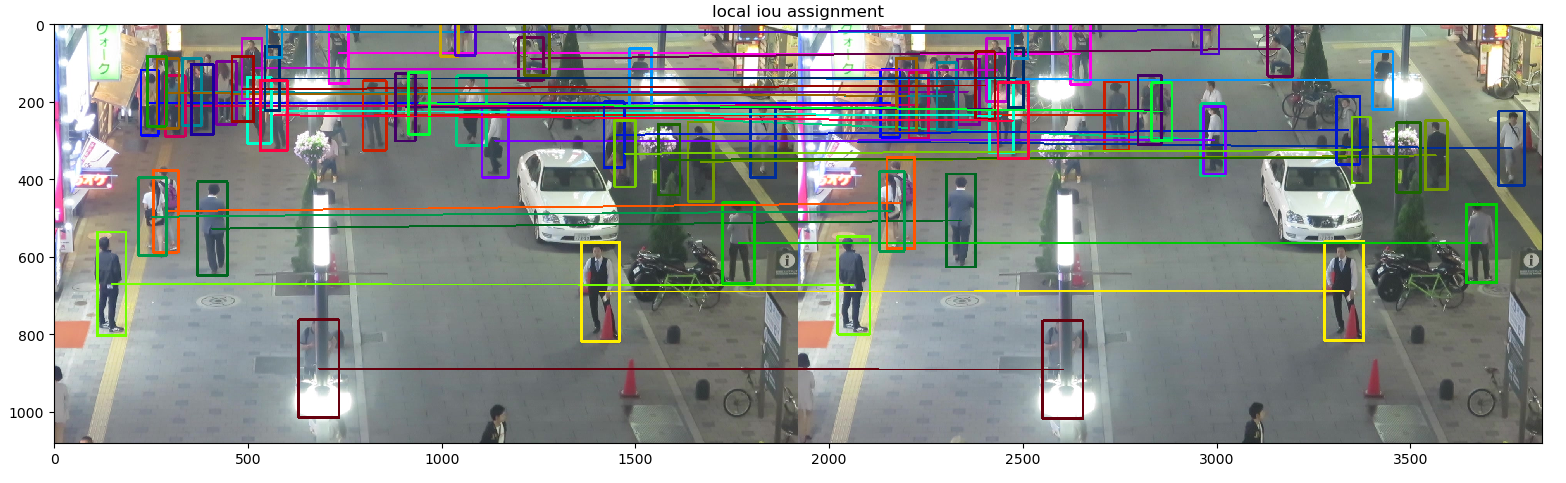
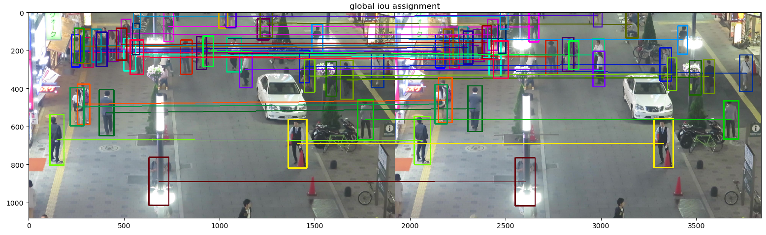
可以看到跟踪效果并不是很差,那么我们观察二者定量的结果则为:

Local: MOTA=0.77, IDF1=0.83

Global: MOTA=0.79, IDF1=0.88

相比之下全局的贪心策略比局部的要好

3 线性分配

3.1 匈牙利算法和KM算法简介

线性分配问题也叫指派问题,通常的线性分配任务是给定N个workers和N个tasks,结合相应的N×N的代价矩阵,就能得到匹配组合。其模型如下:

$$ \begin{array}{l} min = \sum\limits_{i = 1}^N {\sum\limits_{j = 1}^N {{C_{ij}}{x_{ij}}} } \\ s.t.\left\{ \begin{array}{l} \sum\limits_{i = 1}^N {{x_{ij}}} = 1\\ \sum\limits_{j = 1}^N {{x_{ij}}} = 1\\ {x_{ij}} = 0\;or\;1 \end{array} \right. \end{array} $$
上述模型有个问题,即要求workers和tasks的数量对等,然而在MOT问题中待匹配的跟踪轨迹和检测数量大概率不相同,而且我们经常还会设定阈值来限制匹配。

匈牙利算法是专门用来求解指派问题的算法,并且通常用于求解二分图最大匹配的。也就是说我们需要先利用规则判断边是否连接,然后匹配,因此不会出现非边节点存在匹配,只有可能出现剩余未匹配:

$$ \begin{array}{l} max = \sum\limits_{i = 1}^N {\sum\limits_{j = 1}^M {{L_{ij}}{x_{ij}}} } \\ s.t.\left\{ \begin{array}{l} \sum\limits_{i = 1}^N {{x_{ij}}} \le 1\\ \sum\limits_{j = 1}^M {{x_{ij}}} \le 1\\ {x_{ij}} = 0\;or\;1 \end{array} \right. \end{array} $$
匈牙利算法的问题在于一旦确定边之后就没有相对优劣了,所以我们这里介绍带权二分图匹配KM,顾名思义,就是求最小代价,只不过是不对等匹配:

$$ \begin{array}{l} min = \sum\limits_{i = 1}^N {\sum\limits_{j = 1}^M {{C_{ij}}{x_{ij}}} } \\ s.t.\left\{ \begin{array}{l} \sum\limits_{i = 1}^N {{x_{ij}}} {\rm{ = }}1\\ \sum\limits_{j = 1}^M {{x_{ij}}} \le 1\\ {x_{ij}} = 0\;or\;1 \end{array} \right. \end{array} $$
这里我们可以看到有一个维度的和要求是1,原因就是必须要保证有一个维度满分配,不然就会直接不建立连接了。

3.2 实验对比

这里我们借用scipy工具箱实现:

1
2
3
4
5
6
7
8
9
10
11
12
13
14
15
16
17
18
19
20
21
22
23
24
25
26
27
28
29
30
31
32
33
34
35
36
37
38
39
40
41
42
43
44
45
46
47
48
49
50
51
52
53
54
inf_cost = 1e+5

def LinearAssignment(cost, threshold = None, method = 'KM'):
"""Using Hungarian or KM algorithm to make linear assignment

Parameters
----------
cost : ndarray
A NxM matrix for costs between each track_ids with dection_ids
threshold: float
if cost > threshold, then will not be considered
method : str
'KM': weighted assignment
'Hungarian': 01 assignment

Returns
-------
row_idx: List of matched tracks (<=N,)
assigned tracklets' id
col_idx: List of matched dets (<=M,)
assigned dets' id
unmatched_rows: List of unmatched tracks
unassigned tracklets' id
unmatched_cols: List of unmatched dets
unassigned dets' id
min_cost: float
cost of assignments
"""
cost_c = deepcopy(np.atleast_2d(cost))
sz = cost_c.shape

if threshold is not None:
cost_c = np.where(cost_c > threshold, inf_cost, cost_c)

if method == 'Hungarian':
t = threshold if threshold is not None else inf_cost
cost_c = np.where(cost_c < t, 0, cost_c)

# linear assignment
row_ind, col_ind = linear_sum_assignment(cost_c)
if threshold is not None:
t = inf_cost - 1 if threshold == inf_cost else threshold
mask = cost_c[row_ind, col_ind] <= t
row_idx = row_ind[mask]
col_idx = col_ind[mask]
else:
row_idx, col_idx = row_ind, col_ind

unmatched_rows = np.array(list(set(range(sz[0])) - set(row_idx)))
unmatched_cols = np.array(list(set(range(sz[1])) - set(col_idx)))

min_cost = cost[row_idx, col_idx].sum()

return row_idx, col_idx, np.sort(unmatched_rows), np.sort(unmatched_cols), min_cost

同样地,为了更好地对比,我们以IOU为代价指标,分别以匈牙利算法和KM算法为数据关联算法进行实验,有意思的是对于MOT-04-SDP视频而言,二者并没有太大区别,整体效果跟Global IOU Assignment一致。
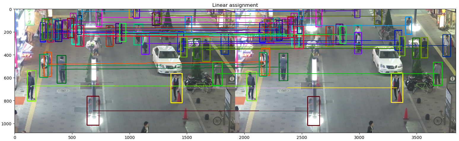
linear_assignment

以上代码我都放到了github

-------------本文结束感谢您的阅读-------------
坚持原创技术分享,您的支持将鼓励我继续创作!