Kalman滤波在MOT中的应用(三)——实践篇


前言

Kalman滤波器是多目标跟踪任务中一个经典的运动模型,本次主要以代码实践进行讲解。下文中所有的代码都会开源在https://github.com/nightmaredimple/libmot。

1Kalman Filter

本章将结合Kalman理论部分进行讲述,Kalman滤波器主要分为预测和更新两个阶段,在这之前能,我们需要预先设定状态变量和观测变量维度、协方差矩阵、运动形式和转换矩阵

1
2
3
4
5
6
7
8
9
10
11
12
13
14
15
16
17
18
19
20
21
22
23
24
25
26
27
28
29
30
31
32
33
34
35
36
37
38
39
40
41
42
43
44
45
46
47
48
49
50
51
52
53
54
55
56
57
58
def __init__(self, dim_x, dim_z, dim_u = 0, x = None, P = None,
Q = None, B = None, F = None, H = None, R = None):
"""Kalman Filter
Refer to http:/github.com/rlabbe/filterpy

Method
-----------------------------------------
Predict | Update
-----------------------------------------
| K = PH^T(HPH^T + R)^-1
x = Fx + Bu | y = z - Hx
P = FPF^T + Q | x = x + Ky
| P = (1 - KH)P
-----------------------------------------
note: In update unit, here is a more numerically stable way: P = (I-KH)P(I-KH)' + KRK'

Parameters
----------
dim_x: int
dims of state variables, eg:(x,y,vx,vy)->4
dim_z: int
dims of observation variables, eg:(x,y)->2
dim_u: int
dims of control variables,eg: a->1
p = p + vt + 0.5at^2
v = v + at
=>[p;v] = [1,t;0,1][p;v] + [0.5t^2;t]a
"""

assert dim_x >= 1, 'dim_x must be 1 or greater'
assert dim_z >= 1, 'dim_z must be 1 or greater'
assert dim_u >= 0, 'dim_u must be 0 or greater'

self.dim_x = dim_x
self.dim_z = dim_z
self.dim_u = dim_u

# initialization
# predict
self.x = np.zeros((dim_x, 1)) if x is None else x # state
self.P = np.eye(dim_x) if P is None else P # uncertainty covariance
self.Q = np.eye(dim_x) if Q is None else Q # process uncertainty for prediction
self.B = None if B is None else B # control transition matrix
self.F = np.eye(dim_x) if F is None else F # state transition matrix

# update
self.H = np.zeros((dim_z, dim_x)) if H is None else H # Measurement function z=Hx
self.R = np.eye(dim_z) if R is None else R # observation uncertainty
self._alpha_sq = 1. # fading memory control
self.z = np.array([[None] * self.dim_z]).T # observation
self.K = np.zeros((dim_x, dim_z)) # kalman gain
self.y = np.zeros((dim_z, 1)) # estimation error
self.S = np.zeros((dim_z, dim_z)) # system uncertainty, S = HPH^T + R
self.SI = np.zeros((dim_z, dim_z)) # inverse system uncertainty, SI = S^-1

self.inv = np.linalg.inv
self._mahalanobis = None # Mahalanobis distance of measurement
self.latest_state = 'init' # last process name

上述即对Kalman滤波器中各个参数的初始化,一般各个协方差矩阵都会初始化为单位矩阵,因此具体的矩阵初始化还需要针对特定场景设计,会在下一章介绍。

然后进入预测环节,这里我们为了保证通用性,引入了遗忘系数$\alpha$,其作用在于调节对过往信息的依赖程度,$\alpha$越大对历史信息的依赖越小。

$$ \begin{array}{l}x = Fx + Bu\\P = \alpha FxF^T + Q\end{array} $$
相应的代码如下:

1
2
3
4
5
6
7
8
9
10
11
12
13
14
15
16
17
18
19
20
21
22
23
24
25
26
27
28
29
30
31
32
33
34
35
36
37
38
39
40
41
42
43
44
def predict(self, u = None, B = None, F = None, Q = None):
"""
Predict next state (prior) using the Kalman filter state propagation equations:
x = Fx + Bu
P = fading_memory*FPF^T + Q

Parameters
----------

u : ndarray
Optional control vector. If not `None`, it is multiplied by B
to create the control input into the system.

B : ndarray of (dim_x, dim_z), or None
Optional control transition matrix; a value of None
will cause the filter to use `self.B`.

F : ndarray of (dim_x, dim_x), or None
Optional state transition matrix; a value of None
will cause the filter to use `self.F`.

Q : ndarray of (dim_x, dim_x), scalar, or None
Optional process noise matrix; a value of None will cause the
filter to use `self.Q`.
"""

if B is None:
B = self.B
if F is None:
F = self.F
if Q is None:
Q = self.Q
elif np.isscalar(Q):
Q = np.eye(self.dim_x) * Q

# x = Fx + Bu
if B is not None and u is not None:
self.x = F @ self.x + B @ u
else:
self.x = F @ self.x

# P = fading_memory*FPF' + Q
self.P = self._alpha_sq * (F @ self.P @ F.T) + Q
self.latest_state = 'predict'

而对于更新阶段,有:

$$ \left\{ \begin{array}{l} K = PH^T/\left( {HPH^T + R} \right)\\ x = Hx + K\left( {z - Hx} \right)\\ P = (1 - KH)P \end{array} \right. $$
不过在实际工程应用中通常会做一些微调:

$$ P = \left( {1 - KH} \right)P{\left( {1 - KH} \right)^T} + KR{K^T} $$

1
2
3
4
5
6
7
8
9
10
11
12
13
14
15
16
17
18
19
20
21
22
23
24
25
26
27
28
29
30
31
32
33
34
35
36
37
38
39
40
41
42
43
44
45
46
47
48
49
50
51
52
53
54
55
56
57
58
59
60
61
62
63
64
65
66
67
68
69
70
71
72
73
def update(self, z, R = None, H = None):
"""
Update Process, add a new measurement (z) to the Kalman filter.
K = PH^T(HPH^T + R)^-1
y = z - Hx
x = x + Ky
P = (1 - KH)P or P = (I-KH)P(I-KH)' + KRK'

If z is None, nothing is computed.

Parameters
----------
z : (dim_z, 1): array_like
measurement for this update. z can be a scalar if dim_z is 1,
otherwise it must be convertible to a column vector.

R : ndarray, scalar, or None
Optionally provide R to override the measurement noise for this
one call, otherwise self.R will be used.

H : ndarray, or None
Optionally provide H to override the measurement function for this
one call, otherwise self.H will be used.
"""

if z is None:
self.z = np.array([[None] * self.dim_z]).T
self.y = np.zeros((self.dim_z, 1))
return

z = reshape_z(z, self.dim_z, self.x.ndim)

if R is None:
R = self.R
elif np.isscalar(R):
R = np.eye(self.dim_z) * R

if H is None:
H = self.H

if self.latest_state == 'predict':
# common subexpression for speed
PHT = self.P @ H.T

# S = HPH' + R
# project system uncertainty into measurement space
self.S = H @ PHT + R

self.SI = self.inv(self.S)


# K = PH'inv(S)
# map system uncertainty into kalman gain
self.K = PHT @ self.SI

# P = (I-KH)P(I-KH)' + KRK'
# This is more numerically stable and works for non-optimal K vs
# the equation P = (I-KH)P usually seen in the literature.
I_KH = np.eye(self.dim_x) - self.K @ H
self.P = I_KH @ self.P @ I_KH.T + self.K @ R @ self.K.T


# y = z - Hx
# error (residual) between measurement and prediction
self.y = z - H @ self.x

self._mahalanobis = math.sqrt(float(self.y.T @ self.SI @ self.y))

# x = x + Ky
# predict new x with residual scaled by the kalman gain

self.x = self.x + self.K @ self.y
self.latest_state = 'update'

其中我们可以注意到马氏距离的计算方式:

1
self._mahalanobis = math.sqrt(float(self.y.T @self.SI @ self.y))

另外,我们保存上个阶段的状态,其主要作用在于,第一防止多次更新带来的重复运算,第二防止前一次更新对下一次更新参数造成影响。

2KalmanTracker

那么对于Kalman滤波器的跟踪器设计,我们这里直接借鉴DeepSort的参数设计方案%E2%80%94%E2%80%94%E5%BA%94%E7%94%A8%E7%AF%87/](https://huangpiao.tech/2020/02/29/Kalman滤波在MOT中的应用(二)——应用篇/),因此基于KalmanFilter的设计,需要在初始化阶段之后修改对应的参数:

1
2
3
4
5
6
7
8
9
10
11
12
13
14
15
16
17
18
19
20
21
22
23
24
25
26
27
28
29
30
31
32
33
34
35
36
37
38
39
40
41
42
43
44
45
46
47
48
49
50
51
52
53
54
55
56
57
58
59
60
61
62
63
def __init__(self, box, fading_memory = 1.0, dt = 1.0, std_weight_position = 0.05, std_weight_velocity = 0.00625):
"""Tracking bounding boxes in assumption of uniform linear motion

The 8-dimensional state space

x, y, a, h, vx, vy, va, vh

contains the bounding box center position (x, y), aspect ratio a, height h,
and their respective velocities.

Object motion follows a constant velocity model. The bounding box location
(x, y, a, h) is taken as direct observation of the state space (linear
observation model).

Parameters
--------------
box: array like
1x4 matrix of boxes (x,y,w,h)
fading_memory: float
larger means fading more
dt: float
time step for each update
std_weight_position: float
std for position
std_weight_velocity:flaot
std for velovity

"""
box = np.atleast_2d(box) #1x4

# initialization
self.x_dim = 8
self.z_dim = 4
self.dt = dt

state = self.box2state(box)
state = np.r_[state, np.zeros_like(state)] #8x1

self.F = np.eye(self.x_dim, self.x_dim)
for i in range(self.z_dim):
self.F[i, self.z_dim + i] = self.dt

self._std_weight_position = std_weight_position
self._std_weight_velocity = std_weight_velocity

std = [
2 * self._std_weight_position * state[3][0],
1e-2,
2 * self._std_weight_position * state[3][0],
10 * self._std_weight_velocity * state[3][0],
1e-5,
10 * self._std_weight_velocity * state[3][0]]
covariance = np.diag(np.square(std))

self.H = np.eye(self.z_dim, self.x_dim)

self.kf = KalmanFilter(dim_x = self.x_dim, dim_z = self.z_dim , x = state,
P = covariance, F = self.F, H = self.H)
self.kf.alpha = fading_memory
self._x = self.kf.x
self._mahalanobis = self.kf.mahalanobis

其中,DeepSort对于Q和R的设计中,为了保证各自对目标尺度更加敏感,采用了自适应的方式,即同样的公式应用在每一次跟踪:

1
2
3
4
5
6
7
8
9
10
11
12
13
14
15
16
17
18
19
20
21
22
23
24
25
26
27
28
29
30
31
32
33
34
35
36
37
38
39
40
41
42
43
44
def predict(self):
"""Predict next state (prior) using the Kalman filter state propagation equations:
x = Fx + Bu
P = fading_memory*FPF^T + Q
"""
std_pos = [
self._std_weight_position * self.kf.x[3][0],
1e-2,
self._std_weight_position * self.kf.x[3][0]]
std_vel = [
self._std_weight_velocity * self.kf.x[3][0],
1e-5,
self._std_weight_velocity * self.kf.x[3][0]]
motion_cov = np.diag(np.square(np.r_[std_pos, std_vel]))

self.kf.predict(Q = motion_cov)

def update(self, measurement):
"""
Update Process, add a new measurement (z) to the Kalman filter.
K = PH^T(HPH^T + R)^-1
y = z - Hx
x = x + Ky
P = (1 - KH)P or P = (I-KH)P(I-KH)' + KRK'

Parameters
--------------
measurement: array like
1x4 matrix of boxes (x,y,w,h)

"""
box = np.atleast_2d(measurement) # 1x4
z = self.box2state(box) # 4x1

std = [
self._std_weight_position * self.kf.x[3][0],
1e-1,
self._std_weight_position * self.kf.x[3][0]]
innovation_cov = np.diag(np.square(std))

self.kf.update(z = z, R = innovation_cov)

另外,为了方便多个观测量对Kalman滤波器的多次更新,我加入了一个批处理模块,主要作用有:防止重复更新造成的变量内存改变、消除重复更新参数部分.

1
2
3
4
5
6
7
8
9
10
11
12
13
14
15
16
17
18
19
20
21
22
23
24
25
26
27
28
29
30
31
32
33
34
35
36
37
38
39
40
41
42
43
44
45
46
47
48
49
50
51
52
53
54
55
56
57
def batch_filter(self, zs):
""" Batch processes a sequences of measurements.

Parameters
----------

zs : list-like
list of measurements at each time step `self.dt`. Missing
measurements must be represented by `None`.

Returns
-------

means : np.array((n,dim_x,1))
array of the state for each time step after the update. Each entry
is an np.array. In other words `means[k,:]` is the state at step
`k`.

covariance : np.array((n,dim_x,dim_x))
array of the covariances for each time step after the update.
In other words `covariance[k,:,:]` is the covariance at step `k`.

mahalanobis: np.array((n,1))
array of the mahalanobises for each time step during the update

"""
zs = np.atleast_2d(zs)
n = zs.shape[0]

# mean estimates from Kalman Filter
x_copy = deepcopy(self.kf.x)
means = np.zeros((n, self.x_dim, 1))

# state covariances from Kalman Filter
covariances = np.zeros((n, self.x_dim, self.x_dim))
mahalanobis = np.zeros(n)

std = [
self._std_weight_position * self.kf.x[3][0],
1e-1,
self._std_weight_position * self.kf.x[3][0]]
innovation_cov = np.diag(np.square(std))

if n > 0:
for i, z in enumerate(zs):
self.kf.x = deepcopy(x_copy)

measurement = self.box2state(z) # 4x1
self.kf.update(z = measurement, R = innovation_cov)
means[i, :] = deepcopy(self.kf.x)
if i == 0:
covariances = np.tile(self.kf.P[np.newaxis, :, :],(n,1,1))

mahalanobis[i] = deepcopy(self.kf._mahalanobis)

return (means, covariances, mahalanobis)

3Example

前两章将Kalman滤波器和跟踪器的代码层面都设计好了,接下来我们以MOT17-10数据集为例进行跟踪实验。这里不采用DeepSort的方式,我自己简单搭建了一套流程:

Step1 我们先初始化参数:

1
2
3
4
5
6
7
8
9
track_len = 655               # total tracking length
thresh_det = 0.75 # threshold for detection,this is for SDP detector
thresh_track = chi2inv95[4] # threshold for data association, specifically the mahalanobis distance
fading_memory = 1.14 # fading memory for prediction
dt = 0.15 # time step for prediction
std_weight_position = 0.04 # std of position prediction
std_weight_velocity = 0.05 # std of velocity prediction
patience = 2 # patience for waiting reconnection
min_len = 4 # mininum length of active trajectory

Step2 读取detection和groundtruth文件,筛选出满足行人类别和检测置信度阈值的目标:

1
2
3
4
5
6
7
8
9
# prefetch
gt = np.genfromtxt(dir_path + 'gt\\gt.txt', delimiter = ',')
gt = gt[(gt[:, 0] < track_len)&(gt[:, 6] == 1) , :]
mask = (gt[:, 7] == 1) | (gt[:, 7] == 2) | (gt[:, 7] == 7)
gt = gt[mask].astype(np.int32)

dets = np.genfromtxt(dir_path + 'det\\det.txt', delimiter = ',')
dets = dets[(dets[:, 0] < track_len)&(dets[:, 6] > thresh_det) , :]
dets = dets.astype(np.int32)

Step3 对每个目标新建一个Kalman滤波器,逐一进行预测、更新、数据关联。其中如果数据关联失败的话,对于匹配失败的跟踪轨迹,在一定时间内,我们依旧允许其预测。

1
2
3
4
5
6
7
8
9
10
11
12
13
14
15
16
17
18
19
20
21
22
23
24
25
26
27
28
29
30
31
32
33
34
35
36
37
38
39
40
41
42
43
44
45
46
47
48
49
50
51
52
53
54
55
56
57
58
59
60
61
62
63
64
65
66
67
68
69
70
71
72
73
74
# begin track
total_id = len(dets[dets[:, 0] == 1])
for i, det in enumerate(dets[dets[:, 0] == 1]):
tracks.append({'id' : i + 1, 'pause': 0,
'kf': LinearMotion(det[2:6], fading_memory = fading_memory, \
dt = dt, std_weight_position = std_weight_position, \
std_weight_velocity = std_weight_velocity)
})
record.append([1, i+1, det[2], det[3], det[4], det[5], 1])

for i in range(2, track_len):
det = dets[dets[:, 0] == i]
cost = (thresh_track + 1)*np.ones((len(tracks), len(det)))
save = [None] * len(tracks)

track_copy = deepcopy(tracks)
track_boxes = np.zeros((len(tracks), 4))

# predict
for j, track in enumerate(tracks):
track['kf'].predict()
track_boxes[j] = track['kf'].x

# iou_blocking
if len(tracks) > 0 and len(det) > 0:
keep = iou_blocking(track_boxes, det[:, 2:6], 2*track_boxes[:, 2:])
xs = np.zeros((det.shape[0], tracks[0]['kf'].x_dim, 1))
Ps = np.zeros((det.shape[0], tracks[0]['kf'].x_dim, tracks[0]['kf'].x_dim))
ds = np.zeros(det.shape[0])

# update
for j, track in enumerate(tracks):
xs[keep[j], :, :], Ps[keep[j], :, :], ds[keep[j]] = track['kf'].batch_filter(det[keep[j], 2:6])
save[j] = {'xs': deepcopy(xs), 'Ps': deepcopy(Ps)}
cost[j, keep[j]] = ds[keep[j]]
# data association
row_idx, col_idx, unmatched_rows, unmatched_cols, _ = LinearAssignment(cost, threshold=thresh_track, method = 'KM')
else:
row_idx = []
col_idx = []
unmatched_rows = np.arange(len(tracks))
unmatched_cols = np.arange(len(det))

for r, c in zip(row_idx, col_idx):

tracks[r]['kf'].kf.x = save[r]['xs'][c, :, :]
tracks[r]['kf'].kf.P = save[r]['Ps'][c, :, :]
tracks[r]['pause'] = 0

for r in np.flip(unmatched_rows, 0):
if tracks[r]['pause'] >= patience:
del tracks[r]
else:
tracks[r]= deepcopy(track_copy[r])
tracks[r]['kf'].predict()
tracks[r]['pause'] += 1

for c in unmatched_cols:
tracks.append({'id': total_id + 1, 'pause': 0,
'kf': LinearMotion(det[c, 2:6], fading_memory=fading_memory, \
dt=dt, std_weight_position=std_weight_position, \
std_weight_velocity=std_weight_velocity)
})
total_id += 1

for track in tracks:
if track['pause'] == 0:
record.append([i, track['id'], track['kf'].x[0], track['kf'].x[1],
track['kf'].x[2], track['kf'].x[3], 1])
else:
record.append([i, track['id'], track['kf'].x[0], track['kf'].x[1],
track['kf'].x[2], track['kf'].x[3], 0])

record = np.array(record)

值得注意的是其中的iou_blocking部分,这个模块使我们基于iou mask改进升级的,原本的iou是用来删除iou<0.3的关联边,现在我们可以放宽要求,将不在目标邻域的观测删除:

1
2
3
4
5
6
7
8
9
10
11
12
13
14
15
16
17
18
19
20
21
22
23
24
25
26
27
28
29
30
31
def iou_blocking(tracks, dets, region_shape):
"""Blocking regions for each tracks

Parameters
-----------
tracks: 2-dim ndarray
Nx4 matrix of (x,y,w,h)
dets: 2-dim ndarray
Mx4 matrix of (x,y,w,h)
region_shape: Tuple(w,h) or array-like (Nx2)
region shape for each track

Returns
---------
blocks: ndarray of boolean(NxM)
block sets for each track,
"""

tracks = np.atleast_2d(tracks)
dets = np.atleast_2d(dets)
if not isinstance(region_shape, tuple):
region_shape = np.atleast_2d(region_shape)
else:
region_shape = np.array([[region_shape[0], region_shape[1]]])
region_shape = np.tile(region_shape, (tracks.shape[0], 1))

centers = tracks[:, :2] + tracks[:, 2:]/2.

overlap = iou(np.c_[centers - region_shape/2., region_shape], dets)
keep = overlap > 0
return keep

Step4 我们将轨迹中有效长度较短的轨迹视为无效轨迹:

1
2
3
4
5
6
7
8
9
10
11
12
# post processure
max_id = record[:, 1].flatten().max()
new_record = None
for i in range(1, max_id + 1):
temp = record[record[:, 1] == i]
index = int(temp[:, -1].nonzero()[0][-1])
temp = temp[:(index+1), :-1]
if len(temp) > min_len or temp[-1, 0] == track_len or temp[0, 0] > track_len - min_len - 1:
if new_record is not None:
new_record = np.r_[new_record, temp]
else:
new_record = temp

上述过程呢,我们可以得到以下结果:

DetectionMOTA↑MOTP↑IDF1↑ID Sw.↓
SDP0.6750.2030.518201

可视化效果如下:

image-20200301184848145

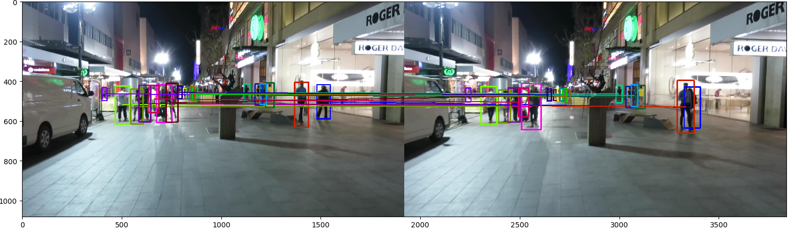
可以看到,在检测质量较好时,跟踪效果也还不错,以上的代码我都放在了https://github.com/nightmaredimple/libmot,


参考资源

[1]WOJKE N, BEWLEY A, PAULUS D. Simple online and realtime tracking with a deep association metric[C]. in: 2017 IEEE international conference on image processing (ICIP). IEEE, 2017. 3645-3649.

[2]https://github.com/rlabbe/filterpy/tree/master/filterpy/

[3]https://github.com/nwojke/deep_sort

-------------本文结束感谢您的阅读-------------
坚持原创技术分享,您的支持将鼓励我继续创作!